
Unit-1: Basic concepts of statistic
INDEX
1.1 population vs. sample, variables (categorical vs. numerical), datatypes.
1.2 Descriptive statistics: measures of central tendency (mean, median, mode),
1.3 Measures of dispersion (range, variance, standard deviation)
NOTES
1.1 Population vs. Sample
🔸 Population
A population in statistics refers to the entire group of individuals, items, or data that you want to study or gather information about.
It can be finite (limited number) or infinite (endless).
A population can include people, objects, events, measurements, etc.
Example:
All students in a college.
Every household in a city.
Every manufactured car in a year.
🔸 Sample
A sample is a smaller group selected from the population.
It is used when studying the whole population is too costly, time-consuming, or impossible.
A sample should be representative, meaning it reflects the characteristics of the population accurately.
Example:
200 students chosen from all students in a college.
1,000 households from a city.
🔸 Key Differences:
| Aspect | Population | Sample |
|---|---|---|
| Size | Complete group | Subset of the population |
| Data Type | Actual values or parameters | Estimates or statistics |
| Cost & Time | High | Less |
| Accuracy | More accurate (if data is available) | Less accurate but manageable |
🔹 Variables: Categorical vs. Numerical
🔸 What is a Variable?
A variable is any characteristic or property that can vary from one individual or item to another.
Variables are mainly classified into two types:
🔹 1. Categorical Variables (Qualitative)
These represent qualities, labels, or categories.
They cannot be measured with numbers.
Can be divided into:
Nominal: No specific order (e.g., gender, blood group, city names)
Ordinal: Ordered categories (e.g., grades like A, B, C or rankings)
Example:
Eye color (Blue, Green, Brown)
Type of vehicle (Car, Bike, Truck)
🔹 2. Numerical Variables (Quantitative)
These represent measurable quantities or values.
Can be used in mathematical calculations.
Two subtypes:
Discrete: Countable values (e.g., number of students, number of cars)
Continuous: Can take any value in a range (e.g., height, weight, temperature)
Example:
Age (in years)
Salary (in ₹)
Distance (in km)
🔹 Data Types
🔸 1. Qualitative Data (Categorical)
Describes non-numeric characteristics.
Used for classification.
Example:
Color, Brand name, Occupation.
🔸 2. Quantitative Data (Numerical)
Represents numerical values.
Used for calculations and statistical analysis.
Example:
Marks obtained, Weight, Income.
| Data Type | Description | Example |
|---|---|---|
| Qualitative | Non-numeric, categories | Gender, City, Language |
| Quantitative | Numeric, measurable | Height, Age, Salary |
📘 1.2 Descriptive Statistics: Measures of Central Tendency
🔹 What is Descriptive Statistics?
Descriptive statistics involves summarizing and organizing data so it can be easily understood. It helps us understand the basic features of data by using tools like:
Tables
Graphs
Averages (measures of central tendency)
Measures of spread (like range, variance, etc.)
In this section, we focus on measures of central tendency.
🔸 Measures of Central Tendency
The measures of central tendency describe the center or typical value of a dataset. They help identify the value around which most of the data points lie.
The three main measures are:
Mean
Median
Mode
🔹 1. Mean (Average)
🔸 Definition:
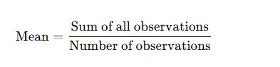
The mean is the sum of all data values divided by the total number of values. It is often called the arithmetic average.
🔸 Formula:
For a data set:
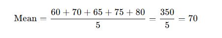
🔸 Example:
Marks of 5 students: 60, 70, 65, 75, 80
🔸 Characteristics:
Affected by extreme values (outliers)
Suitable for quantitative data
🔹 2. Median
🔸 Definition:
The median is the middle value of the data when it is arranged in ascending or descending order.
If the number of observations is odd, the median is the middle number.
If it is even, the median is the average of the two middle numbers.
🔸 Example 1 (Odd number of terms):
Data: 12, 15, 18
Median = 15 (middle value)
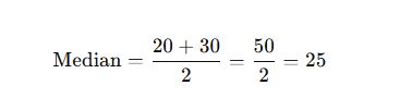
🔸 Example 2 (Even number of terms):
Data: 10, 20, 30, 40
🔸 Characteristics:
Not affected by extreme values
Best used for skewed data or data with outliers
🔹 3. Mode
🔸 Definition:
The mode is the value that occurs most frequently in the dataset.
🔸 Example:
Data: 5, 8, 8, 9, 10
Mode = 8 (since it appears twice)
🔸 Characteristics:
A dataset can have no mode, one mode (unimodal), two modes (bimodal), or more than two modes (multimodal).
Useful for categorical as well as numerical data.
📊 Comparison Table
| Measure | Meaning | Formula/Method | Sensitive to Outliers | Suitable For |
|---|---|---|---|---|
| Mean | Average value | Sum of values ÷ Number of values | Yes | Numerical data |
| Median | Middle value | Middle value in sorted data | No | Skewed data |
| Mode | Most frequent value | Highest frequency value | No | Categorical data |
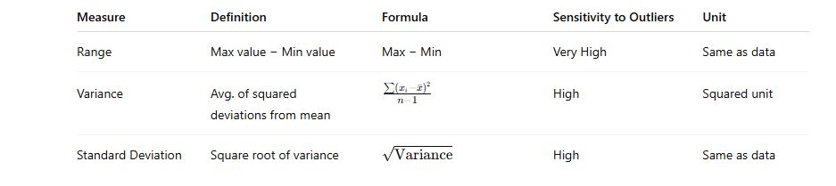
📘 1.3 Measures of Dispersion (Range, Variance, Standard Deviation)
🔹 What is Dispersion in Statistics?
Dispersion refers to the extent to which data values differ from each other and from the central value (mean, median, or mode). It helps to understand how spread out or clustered the data is.
If all values are close to each other, the dispersion is low. If the values are spread out widely, the dispersion is high.
🔸 Types of Measures of Dispersion
There are several methods to measure dispersion. The most commonly used ones are:
Range
Variance
Standard Deviation
🔹 1. Range
🔸 Definition:
The range is the difference between the highest and lowest values in a dataset.
🔸 Formula:
🔸 Example:
Data: 12, 18, 25, 30, 35
Range = 35 – 12 = 23
🔸 Characteristics:
Very simple to calculate.
Affected by extreme values (outliers).
Gives only a rough idea of data spread.
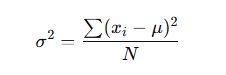
🔹 2. Variance
🔸 Definition:
Variance measures the average squared difference of each data point from the mean. It provides a more detailed understanding of data spread.
🔸 Formula:
For Population Variance (σ²):
For Sample Variance (s²):
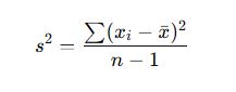
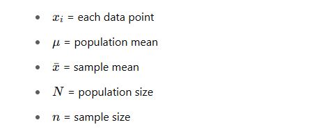
Where:
🔸 Example:
Sample data: 5, 7, 9
Mean = (5 + 7 + 9)/3 = 7
Now:
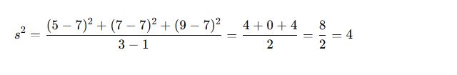
Variance = 4
🔸 Characteristics:
Measures data variability accurately.
Values are always non-negative.
Units are squared (not in the same unit as data).
🔹 3. Standard Deviation
🔸 Definition:
Standard deviation is the square root of variance. It measures the average distance of each data point from the mean.
🔸 Formula:

Using the previous example,
Variance = 4
Standard Deviation = √4 = 2
🔸 Characteristics:
Provides a precise and widely used measure of spread.
Expressed in the same unit as the original data.
A smaller standard deviation means the data is more concentrated around the mean; a larger one means more spread out.
📊 Comparison Table
📝 Conclusion
- Understanding the difference between population and sample, types of variables, and data types is the foundation of statistics. It helps in designing studies, collecting meaningful data, and applying the correct statistical tools for analysis.
- The mean, median, and mode are essential tools in descriptive statistics. They help summarize large data sets with a single representative value, making interpretation easier. Each measure is useful in different situations depending on the type of data and data distribution.
Measures of dispersion are essential in statistics because they show how data is distributed around a central value. While the range gives a basic idea of spread, variance and standard deviation offer a more accurate and meaningful understanding of the variability within a dataset.