
ECONOMICS
CHAPTER 8: Producer’s Equilibrium
8.1 Introduction
The objective of this chapter is to determine the “Equilibrium level of Producer”. Just as a consumer aims to maximise satisfaction , a producer aims to maximise his/her satisfaction.
For a producer, satisfaction is maximised in terms of profit. Therefore, this chapter deals with finding the level of output that yields the maximum profit.
8.2 Meaning of Profit
Profit refers to the excess of receipts from the sale of goods over the expenditure incurred on producing them.
The amount received from the sale of goods is called revenue.
The expenditure on production is called cost.
The difference between revenue and cost is profit
Profit = Revenue – Cost
Profit is the excess of total revenue (TR) over total cost (TC).
Formula
Profit = 𝑇𝑅 − 𝑇𝐶
Profit=TR−TC
Where:
Total Revenue (TR) = Price × Quantity
Total Cost (TC) = Total Fixed Cost (TFC) + Total Variable Cost (TVC)
Types of Profit
Gross Profit
Gross Profit = 𝑇𝑅 − 𝑇𝑉𝐶
Gross Profit=TR−TVC
(It excludes fixed costs)
Net Profit
Net Profit = 𝑇𝑅 −𝑇𝐶
Net Profit=TR−TC
(Includes both fixed and variable costs)
Normal Profit
Minimum return necessary to keep the producer in business
Considered part of cost
Supernormal Profit
Profit above normal profit
8.3 Producer’s Equilibrium
Equilibrium refers to a state of rest where no change is required.
A firm (producer) is in equilibrium when it has no inclination to expand or contract its output.
This state either reflects maximum profits or minimum losses.
Producer’s Equilibrium is that price and output combination which brings the maximum profit to the producer, and profit declines as more is produced.
Methods for Determination of Producer’s Equilibrium:
1. Total Revenue and Total Cost Approach (TR-TC Approach).
2. Marginal Revenue and Marginal Cost Approach (MR-MC Approach)
Situations for Equilibrium:
When Price remains Constant: This occurs under Perfect Competition, where the firm must accept the same price as determined by the industry.
When Price Falls with a rise in output: This occurs under Imperfect Competition, where the firm must reduce the price to increase sales.
The Marginal Revenue – Marginal Cost Approach (MR-MC)
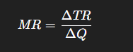
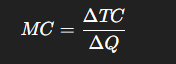
The MR-MC approach is based on comparing the Marginal Revenue (MR) with the Marginal Cost (MC) at different levels of output. Marginal Revenue (MR) is the addition to Total Revenue (TR), and Marginal Cost (MC) is the addition to Total Cost (TC) from producing one more unit.
According to the MR-MC approach, producer’s equilibrium is the output level at which two conditions are satisfied.
Condition 1: Marginal Cost must be Equal to Marginal Revenue
MC = MR (Necessary Condition)
A producer aims to maximize total profits by comparing MR with MC.
Profits increase as long as MR exceeds MC.
Profits fall if MR is less than MC.
Equilibrium is not achieved when MC < MR because the producer can still add to profits by producing more.
The firm is also not in equilibrium when $MC > MR$ because the benefit (MR) is less than the cost (MC).
Thus, the firm is at equilibrium when MC = MR.
Condition 2: MC must be greater than MR after the MC = MR output level
MC > MR after MC = MR output level (Sufficient Condition)
The MC = MR condition is necessary, but not sufficient, as it may occur at more than one output level.
The equilibrium output level must be one where MC becomes greater than MR immediately after the equality.
If MC is greater than MR after the point of equality, producing beyond it will reduce profits.
If MC were less than MR beyond the equality, the producer could still add to profits by producing more.
This condition is often stated as: The MC curve must cut the MR curve from below.
Producer’s Equilibrium in Practice
When Price remains Constant (Perfect Competition)
Revenue Curves: Price (or AR) remains the same at all levels of output. The revenue from every additional unit (MR) is equal to AR. The AR curve is the same as the MR curve, represented by a horizontal line parallel to the X-axis.
Determination: Equilibrium is determined at the output level (OQ) corresponding to Point K because both conditions are met there: (i) MC = MR; and (ii) MC is greater than MR afterwards. Point R (the first intersection) is not the equilibrium because MC < MR immediately after it.
Relation between Price and MC: Since equilibrium is achieved when MC = MR and AR = MR, it means that Price is equal to MC at the equilibrium level.
When Price Falls with rise in output (Imperfect Competition)
Revenue Curves: The MR curve slopes downward, and AR > MR.
Determination: Equilibrium is determined at the output level (OM) corresponding to Point E.
(i) MC = MR at E43.
(ii) MC is greater than MR after MC=MR output level.
Relation between Price and MC: Since more output can only be sold by reducing prices, Price (or AR) > MR. As MC=MR at equilibrium, it follows that Price is greater than MC at the equilibrium level.
8.4 Marginal Revenue–Marginal Cost (MR–MC) Approach
This is the most important method used in Class 12 Economics.
Definitions
Marginal Revenue (MR):
Revenue earned by producing one more unit.
Marginal Cost (MC):
Increase in cost by producing one additional unit.
MR–MC Equilibrium Conditions
The producer is in equilibrium when:
Condition 1: MR = MC
This ensures that the last unit produced adds equal revenue and cost.
Condition 2: MC curve cuts MR curve from below
This ensures MC rises after MR = MC.
If MC is falling at MR = MC, output is not at profit-maximizing level.
Graphical Explanation
Imagine two curves:
MR curve: Horizontal (under perfect competition)
MC curve: U-shaped
Equilibrium occurs where both intersect, and MC rises.