Unit-2 Advanced SQL

skabra1973@gmail.com

8 months ago

Unit-2 Advanced SQL

SQL : A Brief Overview

SQL (Structured Query Language) is a standard programming language used to interact with relational databases.
It enables users to perform operations like creating, retrieving, updating, and managing data stored in database tables.
SQL is essential for database management and widely used in software development, data analysis, and business intelligence.

Key Features of SQL

Data Definition: Allows users to define and modify database schemas using commands such as CREATE, ALTER, and DROP.
Data Manipulation: Enables data retrieval and modification through commands like INSERT, UPDATE, and DELETE.
Data Control: Manages access and permissions using GRANT and REVOKE.
Transaction Control: Maintains database integrity through commands like COMMIT, ROLLBACK, and SAVEPOINT.
Standardized Language: Supported by most relational database systems, including MySQL, Oracle, PostgreSQL, and SQL Server.

Data types in Oracle

Numeric Data Types

Numeric data types store numeric values, including integers, decimals, and floating-point numbers.

Data Type	Description	Example
1.NUMBER(p, s)	Stores numbers with precision (p) and scale (s).	NUMBER(10, 2) for values up to 10 digits with 2 decimal places. .
2.BINARY_FLOAT	Stores single-precision floating-point numbers.	1.23e4
3.BINARY_DOUBLE	Stores double-precision floating-point numbers.	1.23e-10
4.FLOAT	Stores floating-point numbers, equivalent to NUMBER.	FLOAT(6)

Character Data Types

Character data types store alphanumeric characters, including strings.

Data Type	Description	Example
1.CHAR(n)	Fixed-length character data, up to 2000 bytes.	CHAR(5) stores "abc" as "abc " .
2.VARCHAR2(n)	Variable-length character data, up to 4000 bytes.	VARCHAR2(10) for "Hello".
3.NCHAR(n)	Fixed-length Unicode character data, up to 2000 bytes.	NCHAR(5) for multilingual data.
4.NVARCHAR2(n)	Variable-length Unicode character data, up to 4000 bytes.	NVARCHAR2(10) for multilingual strings.
5.CLOB	Stores large character data, up to 4 GB.	Text documents.	6.NCLOB	Stores large Unicode character data, up to 4 GB.	Multilingual documents.

Date and Time Data Types

Date and time data types store date, time, and timestamp values.

Data Type	Description	Example
1. DATE	Stores date and time values, accurate to the second.	01-JAN-2025 12:00:00 .
2.TIMESTAMP	Stores date and time with fractional seconds.	TIMESTAMP '2025-01-01 12:30:45.123'.
3.TIMESTAMP WITH TIME ZONE	Includes time zone information.	2025-01-01 12:30:45.123 +05:30.
4.TIMESTAMP WITH LOCAL TIME ZONE	Adjusts to the database time zone automatically.	User-defined local time.

Large Object (LOB) Data Types

LOB data types store large unstructured data such as multimedia files.

Data Type	Description	Example
1.BLOB	Binary Large Object, up to 4 GB.	Images, videos .
2.CLOB	Character Large Object, up to 4 GB.	Large text files.
3.NCLOB	National Character Large Object, up to 4 GB.	Multilingual large text.
4.BFILE	Stores binary data in external files.	External image file.

ROWID Pseudo Column and DUAL Table in Oracle

Oracle provides special features like the ROWID pseudo column and the DUAL table, which serve specific purposes in database operations and are widely used in SQL queries. Here’s an in-depth look at both concepts:

ROWID Pseudo Column

Definition: The ROWID pseudo column is a unique identifier for each row in a database table. It represents the physical location of a row in the database storage.

Key Characteristics:

Unique Identifier: Each row in a table has a distinct ROWID.
Immutable: The value of ROWID remains constant for a row unless the row is moved (e.g., via a reorganization or export/import operation).
Hexadecimal Representation: The ROWID is displayed in a base-64 encoded format, such as AAAF9AABAAAAZ4hAAA.
Fast Access: Using ROWID to locate and retrieve rows is faster than using indexed or non-indexed column values.

Structure of ROWID: The `ROWID` is internally divided into four parts:

Object Number: Identifies the database object (e.g., table).
File Number: Specifies the file within the tablespace where the row is stored.
Block Number: Identifies the block containing the row.
Row Number: Indicates the row’s position within the block.

Example Usage:

1. Retrieving ROWID:

SELECT ROWID, EmployeeID, Name
FROM Employees;
This query retrieves the ROWID along with other column values.

2. Using ROWID to Update a Row:

UPDATE Employees
SET Name = ‘John Doe’
WHERE ROWID = ‘AAAF9AABAAAAZ4hAAA’;

3.Deleting a Row Using ROWID:

DELETE FROM Employees
WHERE ROWID = ‘AAAF9AABAAAAZ4hAAA’;

Applications:

Optimizing performance for locating specific rows.
Identifying duplicate rows in a table.
Tracking row changes during data migrations.

DUAL Table

Definition:The DUAL table is a special, single-row, single-column table provided by Oracle. It is primarily used to perform operations that do not involve user-defined tables.

Key Characteristics:

System-Defined: Automatically created in all Oracle databases.
Single Row and Column: Contains one row and one column (DUMMY) with a value of X.
Accessible by All Users: The DUAL table is owned by the SYS schema but can be accessed by any user.

Example Usage:

1. Performing Calculations:

SELECT 2 * 3 AS Result FROM DUAL;

2.Getting the Current Date:

SELECT SYSDATE AS CurrentDate FROM DUAL;

3. Using String Functions:

SELECT UPPER(‘oracle’) AS UpperCase FROM DUAL;

4. Generating Sequences:

SELECT SequenceName.NEXTVAL AS NextValue FROM DUAL;

Why Use the DUAL Table?:

Allows execution of functions, calculations, and expressions independently of any user-defined table.
Acts as a placeholder for queries requiring a FROM clause when no actual table is involved.

Comparison Between ROWID and DUAL

Feature	ROWID	DUAL
1.Purpose	Identifies rows uniquely in a table.	Specific to each row in user-defined tables.
2.SCOPE	Specific to each row in user-defined tables.	System-defined, single-row table.
3.Data	Represents physical row location.	Contains a single value (X).
4.Use Case	Row identification, fast access, tracking.	Calculations, function calls, and sequences.

Oracle Numeric Function

Numeric Function

Basic Arithmetic Functions

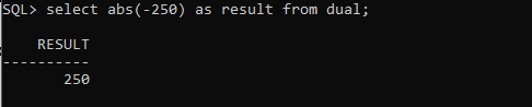
1. ABS() :-

Purpose: Returns the absolute (positive) value of a number.
Syntax: ABS(number)
Example :- select abs(-250) as result from dual;

Basic Arithmetic Functions

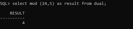
2. MOD :-

Purpose: Returns the remainder of a division operation.
Syntax: MOD(number1, number2)
Example :- select mod (24,5) as result from dual;

Basic Arithmetic Functions

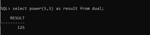
3. POWER :-

Purpose: Raises a number to the power of a specified value.
Syntax: POWER(base, exponent)
Example :- select power(5,3) as result from dual;

Basic Arithmetic Functions

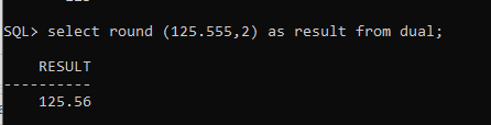
4. ROUND :-

Purpose: Rounds a number to the specified number of decimal places.
Syntax: ROUND(number, decimal_places)
Example :- select round (125.555,2) as result from dual;

Basic Arithmetic Functions

5. TRUNC :-

Purpose: Truncates a number to the specified number of decimal places without rounding.
Syntax: TRUNC(number, decimal_places)
Example :-

Basic Arithmetic Functions

6. CEIL :-

Purpose: Returns the smallest integer greater than or equal to a number.
Syntax: CEIL(number)
Example :- select ceil (125.2) as result from dual;

Basic Arithmetic Functions

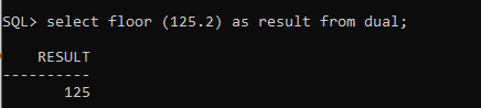
7. FLOOR :-

Purpose: Returns the largest integer less than or equal to a number.
Syntax: FLOOR(number)
Example :- select floor (125.2) as result from dual;

Basic Arithmetic Functions

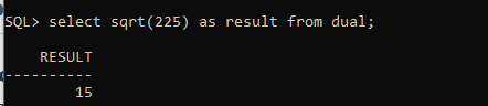
8. SQRT :-

Purpose: Returns the square root of a number.
Syntax: SQRT(number)
Example :- select length(‘WELCOME TO ORACLE 10G’) as result from dual;

Basic Arithmetic Functions

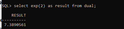
9. EXP :-

Purpose: Returns e raised to the power of the specified number (e ≈ 2.718)..
Syntax: EXP(number)
Example :- select exp(2) as result from dual;

Basic Arithmetic Functions

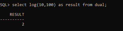
10. LOG

Purpose:- Returns the logarithm of a number to a specified base.
Syntax: – LOG(base, number)
Example :- select chr(’97’) as result from dual;

String Function

String Manipulation Functions

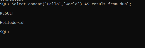
1. CONCAT :-

Purpose: Concatenates two strings.
Syntax: CONCAT(string1, string2)
Example :- Select concat(‘Hello’,’World’) AS result from dual;

TRY YOURSELF

String Manipulation Functions

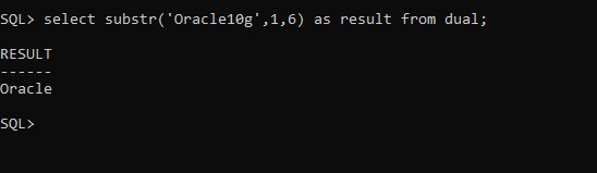
2. SUBSTR :-

Purpose: Extracts a substring from a string.
Syntax: SUBSTR(string, start_position, length)
Example :- select substr(‘Oracle10g’,1,6) as result from dual;

TRY YOURSELF

String Manipulation Functions

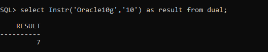
3. INSTR :-

Purpose: Returns the position of a substring within a string.
Syntax: INSTR(string, substring, [start_position], [occurrence])
Example :- select Instr(‘Oracle10g’,’10’) as result from dual;

TRY YOURSELF

String Manipulation Functions

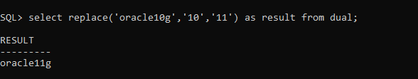
4. REPLACE :-

Purpose: Replaces occurrences of a substring within a string.
Syntax: REPLACE(string, search_string, replacement_string)
Example :- select replace(‘oracle10g’,’10’,’11’) as result from dual;

TRY YOURSELF

String Manipulation Functions

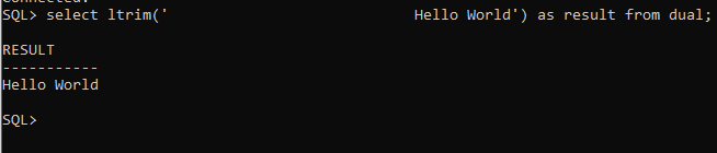
5. LTRIM :-

Purpose: Removes leading characters from a string.
Syntax: LTRIM(string, trim_string)
Example :- select ltrim(‘ Hello World’) as result from dual;

TRY YOURSELF

String Manipulation Functions

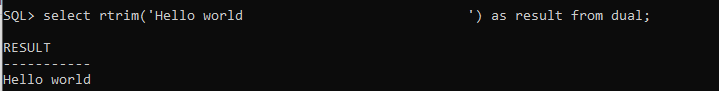
6. RTRIM :-

Purpose: Removes trailing characters from a string..
Syntax: RTRIM(string, trim_string)
Example :- select rtrim(‘Hello world ‘) as result from dual;

TRY YOURSELF

String Manipulation Functions

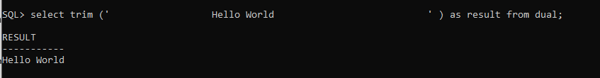
7. TRIM :-

Purpose: Removes leading and trailing characters from a string.
Syntax: TRIM([LEADING|TRAILING|BOTH] trim_char FROM string)
Example :- select trim (‘ Hello World ‘ ) as result from dual;

TRY YOURSELF

String Manipulation Functions

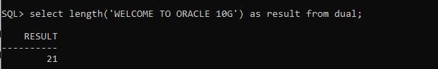
8. LENGTH :-

Purpose: Returns the length of a string.
Syntax: LENGTH(string)
Example :- select length(‘WELCOME TO ORACLE 10G’) as result from dual;

TRY YOURSELF

String Manipulation Functions

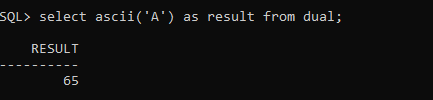
9. ASCII :-

Purpose: Returns the ASCII value of the first character of a string.
Syntax: ASCII(character)
Example :- select ascii(‘A’) as result from dual;

TRY YOURSELF

String Manipulation Functions

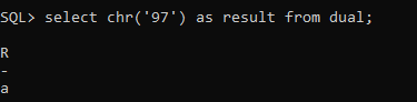
10. CHR :-

Purpose: Returns the character corresponding to an ASCII value.
Syntax: RTRIM(string, trim_string)
Example :- select chr(’97’) as result from dual;

TRY YOURSELF

String Manipulation Functions

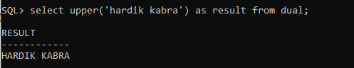
11. UPPER :-

Purpose: Converts a string to uppercase.
Syntax: UPPER(string)
Example :- select upper(‘hardik kabra’) as result from dual;

TRY YOURSELF

String Manipulation Functions

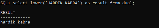
12. Lower :-

Purpose: Converts a string to lowercase.
Syntax: LOWER(string)
Example :- select lower(‘HARDIK KABRA’) as result from dual;

TRY YOURSELF

String Manipulation Functions

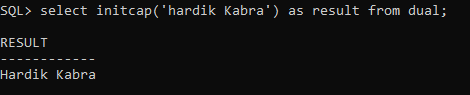
13. INIT :-

Purpose: Converts the first letter of each word in a string to uppercase.
Syntax: INITCAP(string)
Example :- select initcap(‘hardik Kabra’) as result from dual;

TRY YOURSELF

Time and Date Function

Time and Date functions

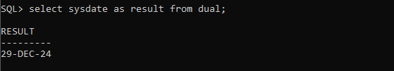
1. SYSDATE :-

Purpose: Returns the current system date and time.
Syntax: SYSDATE
Example :-select sysdate as result from dual;

TRY YOURSELF

Time and Date functions

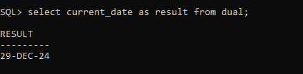
2. CURRENT_DATE :-

Purpose: Returns the current date and time in the session’s time zone.
Syntax: CURRENT_DATE
Example :- select current_date as result from dual;

TRY YOURSELF

Time and Date functions

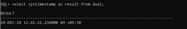
3. SYSTIMESTAMP :-

Purpose: Returns the current system date and time, including time zone information.
Syntax: SYSTIMESTAMP
Example :- select systimestamp as result from dual;

TRY YOURSELF

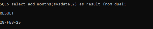
Time and Date functions

4. ADD_MONTHS :-

Purpose: Adds a specified number of months to a date.
Syntax: ADD_MONTHS(date, number_of_months)
Example :- select add_months(sysdate,2) as result from dual;

TRY YOURSELF

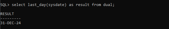
Time and Date functions

5. LAST_DAY :-

Purpose:- Returns the last day of the month for a specified date.
Syntax:- LAST_DAY(date)
Example :- select last_day(sysdate) as result from dual;

TRY YOURSELF

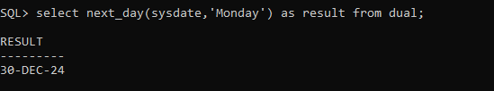
Time and Date functions

6. NEXT_DAY :-

Purpose:- Returns the next date after the given date that falls on a specified weekday.
Syntax:- NEXT_DAY(date, ‘weekday’)
Example :- select next_day(sysdate,’Monday’) as result from dual;

TRY YOURSELF

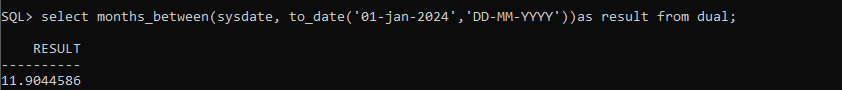
Time and Date functions

7. MONTHS_BETWEEN :-

Purpose:- Calculates the number of months between two dates.
Syntax:- MONTHS_BETWEEN(date1, date2)
Example :- select months_between(sysdate, to_date(’01-jan-2026′,’DD-MM-YYYY’))as result from dual;

TRY YOURSELF

Time and Date functions

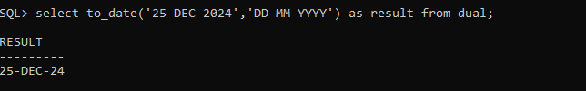
8. TO_DATE :-

Purpose: Converts a string into a date using a specified format.
Syntax: TO_DATE(string, format)
Example :- select to_date(’25-DEC-2024′,’DD-MM-YYYY’) as result from dual;

TRY YOURSELF

Concepts of Index (Create and Drop)

An index in a database is a performance optimization tool that allows for faster retrieval of data.
It acts as a pointer to the data stored in a table, much like an index in a book.
Indexes are especially useful for speeding up queries involving SELECT statements, WHERE clauses, and JOIN operations.

Creating an Index

To create an index, a database management system (DBMS) provides specific commands.
Indexes can be created on one or more columns of a table to optimize specific queries.

1. Syntax for Creating an Index:

CREATE INDEX index_name ON table_name (column1, column2, …);

Example :- CREATE INDEX idx_customer_name ON customers (last_name);

2. Types of Indexes:

1. Unique Index:

Ensures that all values in the indexed column(s) are unique.
CREATE UNIQUE INDEX idx_unique_email ON users (email);

2. Composite Index:

Created on multiple columns to optimize multi-column searches.
CREATE INDEX idx_order_date ON orders (order_date, customer_id);

3. Clustered and Non-Clustered Indexes:

Clustered Index: Sorts the physical data rows in the table based on the indexed column(s). A table can have only one clustered index.
Non-Clustered Index: Creates a separate structure to store the index, with pointers to the table’s data rows.

Dropping an Index

If an index is no longer needed or negatively affects database performance, it can be removed using the DROP INDEX command.
Syntax for Dropping an Index: DROP INDEX index_name ON table_name;
Example: DROP INDEX idx_customer_name ON customers;

Considerations:

Dropping an index may slow down queries that rely on it.
Dropping an index may slow down queries that rely on it.

Benefits of Indexing:

Speeds up data retrieval.
Improves query performance, especially for large datasets.

Drawbacks:

Indexes consume additional storage space.
May slow down write operations (INSERT, UPDATE, DELETE) as the index needs to be updated.

Creating and managing indexes is an essential part of database optimization, requiring careful planning to balance query performance and resource usage.

Join Queries in Oracle

In Oracle databases, join queries are used to retrieve data from multiple tables by combining rows based on a related column between them. Joins are essential for querying relational databases, as they allow for a comprehensive view of data spread across different tables.

Types of Joins in Oracle

1. Inner Join

Returns only the rows that have matching values in both tables.

Syntax:

SELECT columns FROM table1 INNER JOIN table2 ON table1.column = table2.column;

Example:

SELECT employees.name, departments.department_name
FROM employees
INNER JOIN departments
ON employees.department_id = departments.department_id;

2. Outer Join:

Includes rows from one or both tables that do not have matching rows in the other table.

Types:

Left Outer Join:

Returns all rows from the left table and matching rows from the right table.
SELECT columns
FROM table1
LEFT OUTER JOIN table2
ON table1.column = table2.column;

Right Outer Join:

Returns all rows from the right table and matching rows from the left table.
SELECT columns
FROM table1
RIGHT OUTER JOIN table2
ON table1.column = table2.column;

Full Outer Join:

Returns all rows when there is a match in either table.
SELECT columns
FROM table1
FULL OUTER JOIN table2
ON table1.column = table2.column;

3. Cross Join :

Produces a Cartesian product of the two tables, combining each row from the first table with every row from the second table.

Syntax:

SELECT columns
FROM table1
CROSS JOIN table2;

Example:

SELECT employees.name, departments.department_name
FROM employees
CROSS JOIN departments;

4. Self Join

A table is joined with itself to compare rows within the same table.

Syntax:

SELECT A.column, B.column
FROM table A, table B
WHERE A.common_column = B.common_column;

Example:

SELECT A.employee_id, B.manager_id
FROM employees A
INNER JOIN employees B
ON A.manager_id = B.employee_id;

5. Natural Join :

Automatically joins tables based on columns with the same name and datatype.

Syntax:

SELECT columns
FROM table1
NATURAL JOIN table2;

Considerations for Join Queries

Performance: Proper indexing can significantly improve the performance of join queries.
Aliasing: Using table aliases improves readability and prevents ambiguity in queries.
Filtering: Adding WHERE clauses can reduce the result set and improve efficiency.

Subqueries in Oracle

Subqueries with INSERT, UPDATE, and DELETE in Oracle.

A subquery in Oracle is a query nested within another SQL statement.
It is used to retrieve intermediate data that can be used by the main query for various operations like INSERT, UPDATE, or DELETE.
Subqueries can enhance the flexibility and functionality of SQL commands.

1. Subqueries with INSERT

Subqueries can be used with the INSERT statement to populate a table with data retrieved from another table.

Syntax:

INSERT INTO target_table (column1, column2, …)
SELECT column1, column2, …
FROM source_table
WHERE condition;

Example:

INSERT INTO archived_employees (employee_id, name, department_id)
SELECT employee_id, name, department_id
FROM employees
WHERE status = ‘inactive’;

2. Subqueries with UPDATE

Subqueries can be used in the UPDATE statement to dynamically calculate or fetch new values for updating columns in a table.

Syntax:

UPDATE target_table
SET column1 = (SELECT value_column
FROM source_table
WHERE condition)
WHERE condition;

Example:

UPDATE employees
SET salary = (SELECT AVG(salary)
FROM employees
WHERE department_id = 10)
WHERE department_id = 10;

3. Subqueries with DELETE

Subqueries can be used in the DELETE statement to determine which rows to remove based on conditions involving data from another table.

Syntax:

DELETE FROM target_table
WHERE column IN (SELECT column
FROM source_table
WHERE condition);

Example:

DELETE FROM employees
WHERE department_id IN (SELECT department_id
FROM departments
WHERE location_id = 100);

Types of Subqueries

Single-Row Subquery: Returns a single value, typically used with operators like =, <, or >.
Multiple-Row Subquery: Returns multiple values, typically used with operators like IN or ANY.
Correlated Subquery: Refers to columns in the outer query and is evaluated for each row processed by the main query.

Nested Queries in Oracle

A nested query in Oracle, also known as a subquery, is a query embedded within another SQL query.
It is used to perform intermediate calculations or retrieve data that can be used by the outer query.
Nested queries enhance SQL capabilities by enabling complex data retrieval operations.

Characteristics of Nested Queries

Placement:

Nested queries can be placed in various parts of an SQL statement, such as the SELECT, FROM, WHERE, or HAVING clauses.

Execution:

The nested query is executed first, and its result is passed to the outer query.

Types:

Nested queries can be single-row, multi-row, correlated, or uncorrelated.

Types of Nested Queries

1. Single-Row Nested Queries

Returns a single value (row) to the outer query.
Used with operators like =, <, >, <=, and >=.

Example:

SELECT name
FROM employees
WHERE salary = (SELECT MAX(salary) FROM employees);

2. Multi-Row Nested Queries

Returns multiple rows to the outer query.
Typically used with operators like IN, ANY, or ALL.

Example:

SELECT name
FROM employees
WHERE department_id IN (SELECT department_id FROM departments WHERE location_id = 100);

3. Correlated Nested Queries

Refers to columns in the outer query and is executed repeatedly for each row of the outer query.

Example:

SELECT name
FROM employees e
WHERE salary > (SELECT AVG(salary) FROM employees WHERE department_id = e.department_id);

4. Uncorrelated Nested Queries

Independent of the outer query and executed only once.

Example:

SELECT name
FROM employees
WHERE salary > (SELECT AVG(salary) FROM employees);

Advantages of Nested Queries

Modularity: Breaks down complex operations into smaller, manageable steps.
Reusability: Nested queries can be used across multiple main queries with minimal modification.
Flexibility: Enables sophisticated data retrieval, such as comparisons and filtering across tables.

Best Practices

Performance: Avoid overly complex nested queries that may impact execution time.
Indexes: Use indexes on columns referenced in nested queries to improve efficiency.
Alternative Approaches: Consider joins or common table expressions (CTEs) for better readability and performance when dealing with large datasets.

Feature	ROWID	DUAL
1.Purpose	Identifies rows uniquely in a table.	Specific to each row in user-defined tables.
2.SCOPE	Specific to each row in user-defined tables.	System-defined, single-row table.
3.Data	Represents physical row location.	Contains a single value (X).
4.Use Case	Row identification, fast access, tracking.	Calculations, function calls, and sequences.

DUAL Table

Definition:The DUAL table is a special, single-row, single-column table provided by Oracle. It is primarily used to perform operations that do not involve user-defined tables.

Key Characteristics:

System-Defined: Automatically created in all Oracle databases.
Single Row and Column: Contains one row and one column (DUMMY) with a value of X.
Accessible by All Users: The DUAL table is owned by the SYS schema but can be accessed by any user.

Example Usage:

1. Performing Calculations:

SELECT 2 * 3 AS Result FROM DUAL;

2.Getting the Current Date:

SELECT SYSDATE AS CurrentDate FROM DUAL;

3. Using String Functions:

SELECT UPPER(‘oracle’) AS UpperCase FROM DUAL;

4. Generating Sequences:

SELECT SequenceName.NEXTVAL AS NextValue FROM DUAL;

Why Use the DUAL Table?:

Allows execution of functions, calculations, and expressions independently of any user-defined table.
Acts as a placeholder for queries requiring a FROM clause when no actual table is involved.

Comparison Between ROWID and DUAL

Feature	ROWID	DUAL
1.Purpose	Identifies rows uniquely in a table.	Specific to each row in user-defined tables.
2.SCOPE	Specific to each row in user-defined tables.	System-defined, single-row table.
3.Data	Represents physical row location.	Contains a single value (X).
4.Use Case	Row identification, fast access, tracking.	Calculations, function calls, and sequences.