
Unit-2: Data Representation and Sampling Technique
NOTES
2.1 Graphical Representation of Data
Graphical representation is a visual method to present data. It helps in understanding patterns, trends, and relationships more easily than looking at raw numbers. Common types include histograms, box plots, and scatter plots.
🔹 1. Histogram
Brief Explanation:
A histogram is a bar graph that shows the frequency of numerical data grouped into intervals (called bins). It shows how often data values fall within certain ranges.
Detailed Explanation:
A histogram looks similar to a bar graph but is used for continuous data.
The x-axis shows the class intervals, and the y-axis shows the frequency (how many values fall into each interval).
All bars are touching each other to show the continuous nature of the data.
It helps identify distribution patterns (normal, skewed, etc.)
Example:
If we collect the heights of 100 students and group them into intervals like 140-150 cm, 150-160 cm, etc., a histogram can show how many students fall into each range.
🔹 2. Box Plot (Box and Whisker Plot)
Brief Explanation:
A box plot displays the distribution of a dataset using five-number summaries: minimum, first quartile (Q1), median (Q2), third quartile (Q3), and maximum.
Detailed Explanation:
It shows the spread and skewness of data.
The box shows the middle 50% of the data (from Q1 to Q3).
A line inside the box shows the median (middle value).
“Whiskers” extend to the smallest and largest values that are not outliers.
Outliers are shown as dots or stars outside the whiskers.
Usefulness:
It helps in comparing distributions between multiple groups.
Useful in identifying skewness, spread, and outliers in the data.
🔹 3. Scatter Plot
Brief Explanation:
A scatter plot shows the relationship between two numerical variables using dots on a graph.
Detailed Explanation:
Each point on the graph represents an individual data pair (x, y).
The x-axis represents the independent variable, and the y-axis represents the dependent variable.
Helps in analyzing correlation between variables:
Positive correlation: points go upward
Negative correlation: points go downward
No correlation: points are scattered randomly
Example:
If we plot hours studied (x-axis) and marks obtained (y-axis) for students, we may observe that as study hours increase, marks also increase — showing a positive correlation.
✅ Summary Table
| Graph Type | Data Type | Shows | Usefulness |
|---|---|---|---|
| Histogram | Continuous | Frequency distribution | Understand data spread and shape |
| Box Plot | Continuous | Median, Quartiles, Outliers | Compare data distributions |
| Scatter Plot | Paired numeric | Relationship between variables | Analyze correlation or trends |
2.2 Probability Theory: Basic Probability Concepts
🔹 Brief Explanation:
Probability is a branch of mathematics that deals with the chance or likelihood of an event happening. It helps us to predict how likely it is for something to occur — using numbers between 0 and 1.
🔹 Detailed Explanation:
✅ What is Probability?
Probability is the measure of uncertainty or chance. It tells us how likely an event is to occur.
If an event cannot happen, its probability is 0.
If an event will surely happen, its probability is 1.
For all other cases, the probability lies between 0 and 1.
✅ Important Terms:
| Term | Description |
|---|---|
| Experiment | An action or process that leads to one or more outcomes (e.g., tossing a coin). |
| Sample Space (S) | The set of all possible outcomes of an experiment. |
| Event (E) | A specific outcome or a set of outcomes of interest. |
| Favorable Outcomes | Outcomes that satisfy the condition of the event. |
✅ Basic Probability Formula:

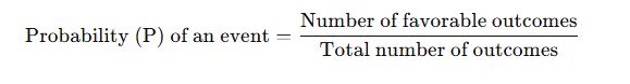
✅ Example:
If a die is rolled, the sample space is {1, 2, 3, 4, 5, 6}.
Let’s find the probability of getting a 4:
Favorable outcomes = 1 (only the number 4)
Total outcomes = 6
✅ Types of Events:
| Type of Event | Explanation |
|---|---|
| Certain Event | An event that is sure to happen (P = 1) |
| Impossible Event | An event that can never happen (P = 0) |
| Equally Likely Events | Events that have the same chance of occurring |
| Mutually Exclusive | Events that cannot happen at the same time |
| Complementary Events | The events “happening” and “not happening” of a particular event (P(E) + P(not E) = 1) |
✅ Real-life Examples:
Tossing a coin (Head or Tail)
Rolling a die (1 to 6)
Drawing a card from a deck (52 cards)

2.3 Probability Distributions (Binomial, Normal Distributions)
🔹 Brief Explanation:
Probability distribution refers to how probabilities are distributed over different possible outcomes of a random experiment. Two widely used types of distributions are:
Binomial Distribution – used when an experiment has only two outcomes (like success/failure).
Normal Distribution – used for data that follows a bell-shaped curve, representing many natural phenomena like height, weight, etc.
🔹 Detailed Explanation:
✅ What is a Probability Distribution?
A probability distribution describes how the probabilities are assigned to the outcomes of a random variable.
There are two main types:
Discrete Probability Distribution – used when the variable takes a countable number of values.
Continuous Probability Distribution – used when the variable can take any value in a range.
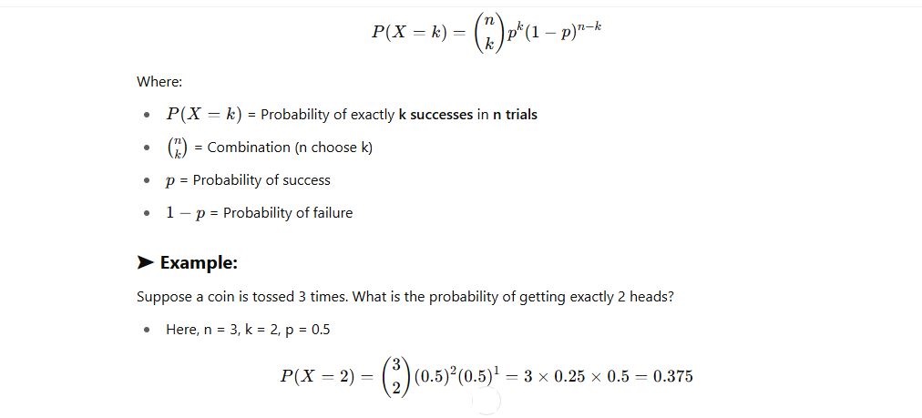
🔸 1. Binomial Distribution
➤ What it is:
Binomial distribution applies when:
An experiment is repeated n times.
Each trial has only two outcomes: success or failure.
The probability of success (p) remains the same in each trial.
The trials are independent of each other.
➤ Formula:

🔸 2. Normal Distribution
➤ What it is:
Normal distribution is a continuous probability distribution that is symmetrical and bell-shaped. It is also called the Gaussian distribution.
➤ Properties:
The mean, median, and mode are all equal and lie at the center.
The curve is symmetrical around the mean.
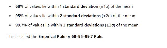
Most of the data lies within ±1, ±2, and ±3 standard deviations from the mean.
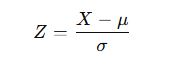
➤ Standard Normal Distribution:
A normal distribution with:
Mean (μ) = 0
Standard Deviation (σ) = 1
It is used to convert normal variables into a standard scale using the Z-score formula

➤ Real-life Examples:
Heights of people
Exam scores
Measurement errors
IQ scores
✅ Comparison Table:
| Feature | Binomial Distribution | Normal Distribution |
|---|---|---|
| Type | Discrete | Continuous |
| Shape | Varies (can be symmetric or skewed) | Bell-shaped and symmetric |
| Trials | Fixed number of trials (n) | Infinite outcomes over a range |
| Outcomes | Two (success/failure) | Continuous values |
| Parameters | n (trials), p (probability of success) | μ (mean), σ (standard deviation) |
| Common Use | Yes/No type experiments | Natural measurements (height, weight, etc.) |
✅ Summary Points:
Binomial Distribution is used when there are a fixed number of repeated independent experiments with two outcomes.
Normal Distribution is useful for data that is naturally distributed and follows a bell-shaped curve.
Both distributions are central to statistics and probability and are widely used in research and data analysis.
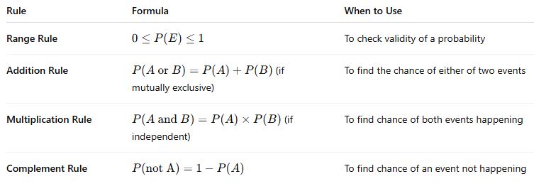
2.4 Rules of Probability
🔹 Brief Explanation:
The rules of probability help us to calculate the chances of single or combined events occurring. The most commonly used rules are:
Addition Rule
Multiplication Rule
Complementary Rule
Range Rule
These rules form the foundation for solving probability problems in real-life and mathematical scenarios.
🔹 Detailed Explanation:
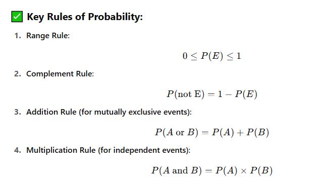
✅ 1. Range Rule of Probability
This rule defines the boundaries within which all probabilities must lie.

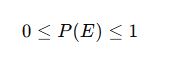
A probability cannot be negative.
The minimum value of probability is 0 (impossible event).
The maximum value is 1 (certain event).
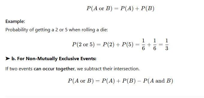
✅ 2. Addition Rule
This rule is used when we are calculating the probability of either one event or another event occurring.
➤ a. For Mutually Exclusive Events:
If two events cannot happen at the same time, they are called mutually exclusive.

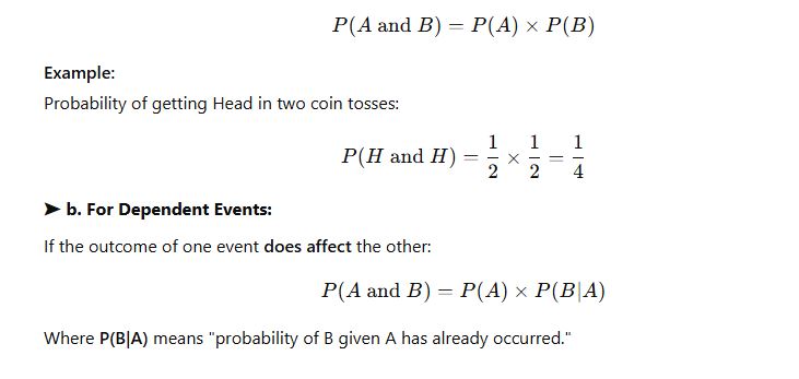
✅ 3. Multiplication Rule
This rule is used when we want to find the probability of two events happening together.
➤ a. For Independent Events:
If the outcome of one event does not affect the other, the events are independent.


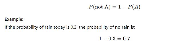
Every event has a complement — the event not happening.

✅ Summary Table:

✅ Real-life Uses:
Games (dice, cards, coins)
Weather prediction
Medical testing
Decision-making in business or finance
2.5 Sampling Techniques: Random Sampling, Stratified Sampling
🔹 Brief Explanation:
Sampling is the process of selecting a small group (called a sample) from a larger group (called a population) to study and draw conclusions. Two common sampling methods are:
Random Sampling – Every individual in the population has an equal chance of being selected.
Stratified Sampling – The population is divided into groups (strata), and samples are taken from each group.
🔹 Detailed Explanation:
✅ What is Sampling?
Sampling is a technique used in statistics to collect data from a subset of a population when it’s not possible or practical to study the whole population.
It helps save time, cost, and effort, while still providing useful information.
🔸 1. Random Sampling
➤ Definition:
In random sampling, each individual or item in the population has an equal and independent chance of being selected.
➤ Features:
Simple to use
Removes selection bias
Ensures fairness in selection
➤ Methods of Random Sampling:
Lottery Method: Names or numbers are written on slips, mixed, and chosen randomly.
Random Number Table or Generator: Using a computer or calculator to pick random numbers.
➤ Example:
If there are 100 students in a school, and we need to select 10 for a survey, using a lottery method to randomly pick any 10 names is random sampling.
➤ Advantages:
Easy to understand and implement
Every member has an equal chance
➤ Disadvantages:
May not represent sub-groups fairly if the population is diverse
🔸 2. Stratified Sampling
➤ Definition:
In stratified sampling, the population is divided into groups (called strata) based on a particular characteristic (like gender, age, class). Then, random samples are taken from each group.
➤ Features:
Ensures all sub-groups are represented
Useful for comparing different groups
➤ Steps Involved:
Divide the population into strata (e.g., male/female, rural/urban).
Select a sample randomly from each group.
Combine all selected samples for final analysis.
➤ Example:
Suppose a college has 200 students – 120 boys and 80 girls. To conduct a survey of 50 students:
Divide the students into two groups (boys and girls).
Take 30 boys (60%) and 20 girls (40%) using random sampling.
This is stratified sampling.
➤ Advantages:
Ensures fair representation of different groups
Gives more accurate results
➤ Disadvantages:
More complex and time-consuming
Requires information about population groups
✅ Comparison Table:
| Feature | Random Sampling | Stratified Sampling |
|---|---|---|
| Basis of Selection | Purely random | Based on specific characteristics (strata) |
| Representation | May not represent all sub-groups | Ensures representation of all sub-groups |
| Complexity | Simple | More detailed and planned |
| Accuracy | Moderate | Higher, especially for diverse populations |
✅ When to Use Which?
Use random sampling when the population is uniform or similar.
Use stratified sampling when the population includes different categories or groups and you want each group fairly represented.
🔹 Brief Explanation:
A sampling distribution is the probability distribution of a statistical measure (like the mean or proportion) calculated from many random samples taken from the same population. It helps us understand how sample statistics behave and vary, even when drawn from the same population.
🔹 Detailed Explanation:
✅ What is a Sampling Distribution?
When we take several random samples from a population and compute a statistic (like mean, median, or proportion) for each sample, we get different values.
A sampling distribution is the distribution (spread or pattern) of these sample statistics.
It tells us:
How the sample mean, proportion, or other statistic behaves across many samples
How much variation we can expect between different samples
How reliable our sample is in estimating the population
✅ Key Concepts:
| Term | Explanation |
|---|---|
| Sample Statistic | A value calculated from sample data (e.g., sample mean, sample proportion) |
| Population Parameter | A value that describes the entire population (e.g., population mean) |
| Sampling Distribution | The distribution of a sample statistic over many repeated samples |
✅ Example:
Imagine a school has 1000 students. Instead of asking all students about their average screen time, you take 30 random samples, each with 50 students, and calculate the average screen time for each sample.
You now have 30 different sample means.
If you plot these means on a graph, the resulting graph shows the sampling distribution of the sample mean.
✅ Importance of Sampling Distribution:
Estimation:
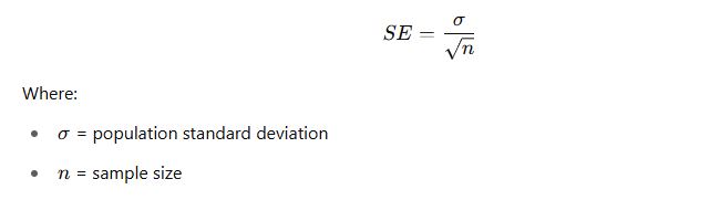
It helps us estimate unknown population parameters using sample data.Standard Error (SE):
The spread of the sampling distribution is called the standard error. A smaller SE means the sample mean is a good estimate of the population mean.

3. Basis for Statistical Inference:
It allows us to perform hypothesis testing and create confidence intervals.
✅ Types of Sampling Distributions:
| Type | Description |
|---|---|
| Sampling distribution of the mean | Distribution of sample means |
| Sampling distribution of the proportion | Distribution of sample proportions |
| Sampling distribution of the difference | Used when comparing two different sample statistics |
✅ Central Limit Theorem (CLT):
The Central Limit Theorem states that:
If you take sufficiently large random samples from any population, the sampling distribution of the sample mean will be approximately normal, even if the population itself is not normal.
✅ Summary Points:
A sampling distribution shows how a sample statistic varies from sample to sample.
It is used to understand and estimate population characteristics.
Standard error measures how much sample statistics differ from the actual population parameter.
The Central Limit Theorem helps explain why sample means tend to follow a normal distribution when sample size is large.
2.7 Understanding Bell Curve
🔹 Brief Explanation:
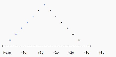
The Bell Curve, also known as the Normal Distribution Curve, is a graph that represents a naturally occurring distribution of data where most values are centered around the mean. It has a symmetrical, bell-shaped appearance, and is widely used in statistics to understand patterns and make predictions.
✅ What is a Bell Curve?
The Bell Curve is the graphical representation of the normal distribution, a type of continuous probability distribution. In this distribution:
Most data points are clustered around the mean.
Fewer and fewer data points lie far away from the mean on either side.
The curve is symmetrical, meaning both sides look the same.
✅ Key Features of the Bell Curve:
| Feature | Description |
|---|---|
| Shape | Symmetrical and bell-shaped |
| Mean = Median = Mode | All three are located at the center of the curve |
| Spread | Controlled by standard deviation (σ), which measures data dispersion |
| Tails | Extend infinitely in both directions but never touch the horizontal axis |
| Area Under Curve | Total area = 1 (or 100%), representing the total probability distribution |
✅ Standard Deviation and the Bell Curve:
In a normal distribution:

✅ Why Is the Bell Curve Important?
Predictability:
It helps predict the likelihood of outcomes in a wide variety of fields like education, psychology, economics, etc.Benchmarking Performance:
It’s used in grading systems, employee performance evaluations, and standardized testing.Quality Control:
Businesses use it to monitor variations in processes or product quality.
✅ Real-Life Examples:
| Scenario | Explanation |
|---|---|
| Heights of people | Most people are of average height; fewer are very tall or very short |
| Exam scores | Most students score near the average; very high or low scores are rare |
| IQ scores | Majority of people have average IQs; extreme values are uncommon |

✅ Summary Points:
The bell curve is the graph of a normal distribution.
It is symmetrical, with most data near the mean.
The mean, median, and mode are all equal and lie at the center.
The curve is used for analyzing trends, making predictions, and evaluating performance.