5.3 Calculating summary statistics (mean, median, mode, standard deviation).
5.4 Generating frequency tables and cross-tabulations.
5.5 Understanding measures of central tendency and dispersion.
5.6 Exploring data distributions graphically (Bell curve).
NOTES
Unit-5: Working with Data in R
🔹 5.1 Reordering and Reshaping Data Frames in R
✅ 1. Introduction
Data in R is mostly stored and manipulated using data frames. During data analysis, it is often necessary to reorder or reshape data to better understand it or prepare it for further analysis, such as plotting or modeling.
🔄 2. Reordering Data Frames
Reordering refers to changing the order of rows or columns in a data frame based on certain criteria.
🧩 a. Reordering Rows
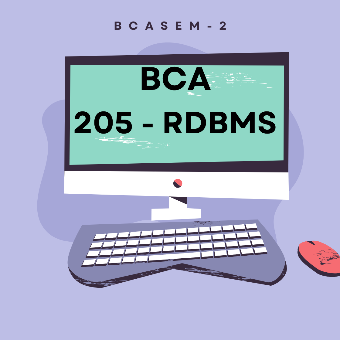
You can reorder rows based on values in a column using the order() function.
Explanation:
order(df$Age) returns the index to sort by age.
df[order(df$Age), ] reorders rows by that column.
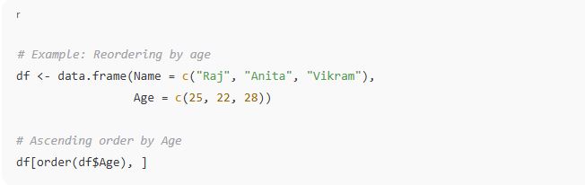
📌 You can also use dplyr package:
🧩 b. Reordering Columns
To reorder columns, you can simply rearrange them using indexing:
🔁 3. Reshaping Data Frames
Reshaping means transforming the structure of a data frame—usually converting it between wide and long formats.
📊 a. Wide Format vs. Long Format
Wide Format: Each subject has a single row. Multiple columns represent different variables or time points.
Long Format: Each observation gets its own row. Columns typically include ID, variable name, and value.
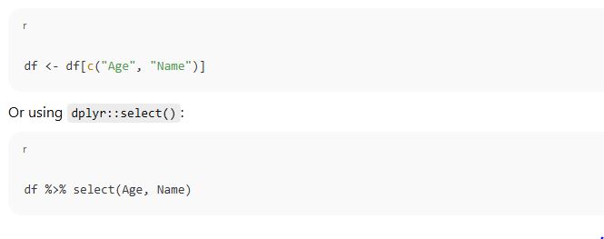
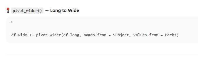
🔁 b. pivot_longer() and pivot_wider() from tidyr
These functions are used for reshaping:
📍 pivot_longer() → Wide to Long
Name
Subject
Marks
Raj
Math
80
Raj
Science
85
Anita
Math
90
Anita
Science
95
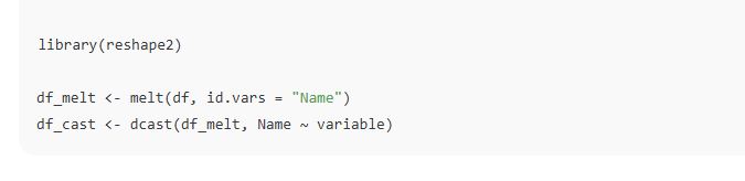
🧩 c. melt() and dcast() from reshape2 package (older)
🎯 4. Why Reordering & Reshaping is Important
Purpose
Benefits
Data Cleaning
Makes large data manageable and readable
Preparation for Visualization
Many plots (like ggplot) require long-format data
Better Analysis
Helps in grouping, summarizing, or comparing data
Model Input
Some models require data in a specific format
Unit 5.2 Merging and Joining Data Frames
✅ 1. Introduction
In real-world data analysis, we often deal with multiple datasets that need to be combined based on common columns or keys. In R, merging or joining data frames allows us to bring related information together into one unified table.
🔁 2. What is Merging or Joining?
Merging or joining means combining two or more data frames using one or more common columns (like IDs, names, or codes).
There are different types of joins depending on how you want to combine the data.
📌 3. Merging Data Frames Using Base R
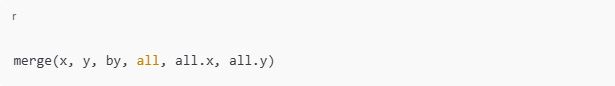
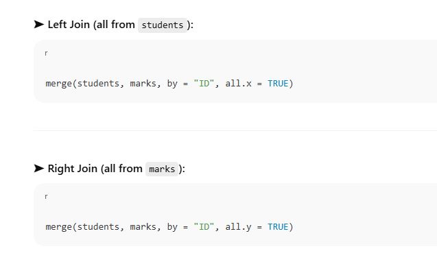
🧩 a. merge() Function
x, y → the data frames to merge
by → the column(s) to merge on
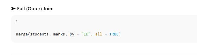
all → if TRUE, performs full outer join
all.x → if TRUE, performs left join
all.y → if TRUE, performs right join
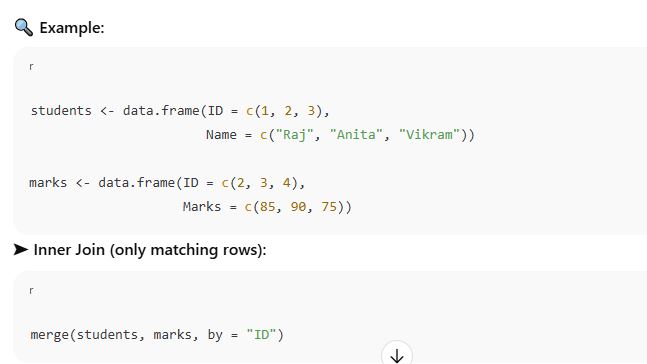
ID
Name
Marks
2
Anita
85
3
Vikram
90
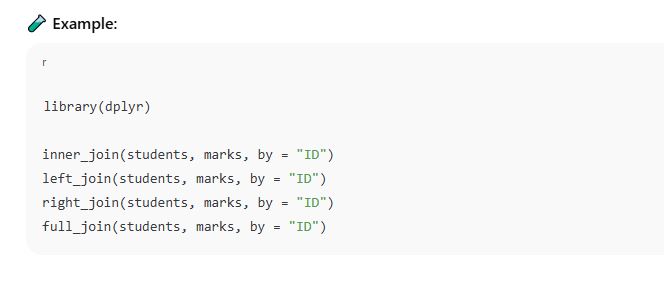
🔧 4. Joining Using dplyr Package (Tidyverse)
The dplyr package provides clear and easy-to-read functions for different types of joins:
Function
Join Type
inner_join()
Inner Join
left_join()
Left Join
right_join()
Right Join
full_join()
Full (Outer) Join
anti_join()
Non-matching rows
semi_join()
Matching rows only from first table
📌 5. Real-World Use Cases
Situation
Join Type
List of customers + their purchases
Left Join
Employee details + attendance records
Inner Join
Sales data + product codes
Full Join
Missing students from marklist
Anti Join
🎯 6. Why is Merging/Joining Important?
Reason
Benefit
Combine Related Datasets
Easier to analyze together
Clean and Prepare Data
Unified structure for modeling/plotting
Fill Missing Info
Add data from other sources
Data Consistency
Ensure all linked records are considered
5.3 Calculating Summary Statistics (Mean, Median, Mode, Standard Deviation)
✅ 1. Introduction
Summary statistics help us understand the basic characteristics of a dataset. In R, we can easily calculate key statistical measures like mean, median, mode, and standard deviation to summarize the data and draw insights.
📌 2. What Are Summary Statistics?
Statistic
Description
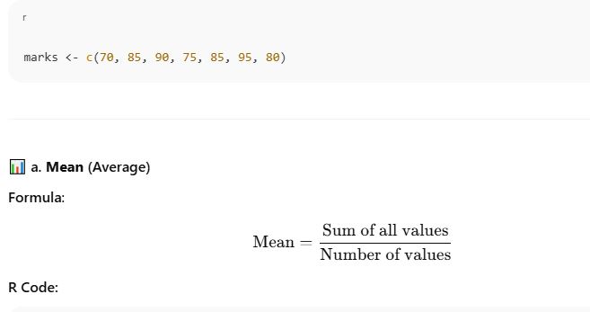
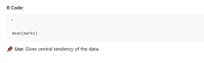
Mean
Average of all values
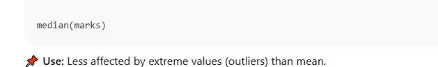
Median
Middle value when data is sorted
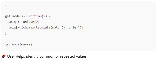
Mode
Most frequently occurring value
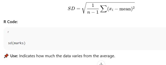
Standard Deviation
Spread or variation of data from the mean
🧮 3. Calculating Summary Statistics in R
Let’s assume we have a dataset of student marks:
📊 b. Median (Middle value)
If the data is odd, it’s the center value. If even, it’s the average of the two middle values.
R Code:
📊 c. Mode (Most frequent value)
R does not have a built-in mode() for numeric data, so we define a custom function:
📊 d. Standard Deviation (Spread of data)
Formula:
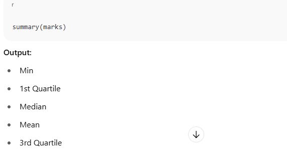
📋 4. Summary of All Statistics Together
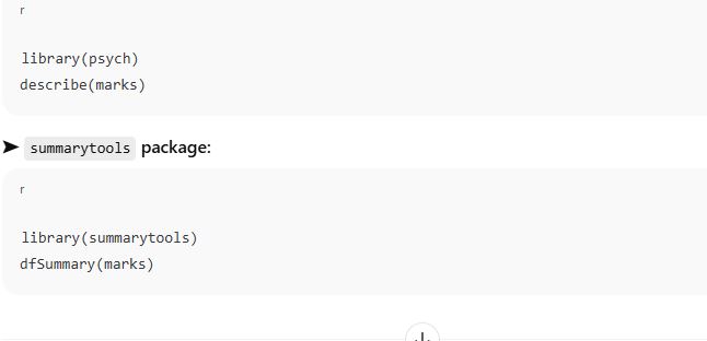
🔧 5. Additional Tools in R
You can also use packages like:
➤ psych package:
🎯 6. Importance of Summary Statistics
Purpose
Benefit
Quick understanding
Gives overview of data distribution
Detect outliers
Median helps find unusual data
Evaluate variability
SD shows consistency in data
Prepare for further analysis
Needed before visualization or modeling
5.4 Generating Frequency Tables and Cross-Tabulations
✅ 1. Introduction
In data analysis, it’s important to understand how often values occur and how variables relate to each other.
Frequency Tables help count the number of times each value appears.
Cross-Tabulations (also called contingency tables) show the relationship between two categorical variables.
R provides built-in and package-based functions to easily generate both.
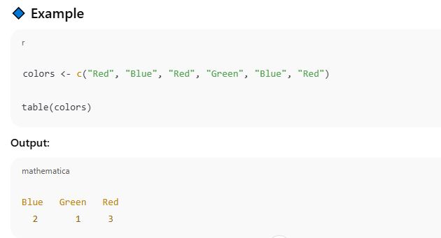
📊 2. Frequency Tables
🔹 What is a Frequency Table?
A frequency table shows the count of each unique value in a variable.